LLM Inference Explained: Weights, Quantization, KV Cache and More
- Gate
- AI & ML
- Departs
- Crew
- [email protected] (Bruno Ferreira)
- Passengers
- 580
A practical guide to LLM memory and inference, from model weights and context limits to retrieval, expert routing and token generation.

Why local LLMs need a new vocabulary
Running a language model on a personal computer brings its inner workings into view. A hosted chatbot hides most of the hardware tradeoffs; a local model makes them hard to ignore. Model size, memory use, response speed and answer quality depend on how the system stores information and processes each request. Nvidia’s RTX Spark is one example of hardware drawing attention to local AI, but the concepts apply across consumer GPUs and other machines that can run text models.
This guide focuses on text-based large language models (LLMs): chat assistants, coding tools and agent-style systems that work through language. The terms also help explain why two models with similar parameter counts can behave differently, why a long conversation can slow down, and why a fast graphics card alone doesn’t guarantee fast responses.
Models, tokens and learned weights
A model is the trained system that maps input text to likely output text. During training, it processes large collections of material, including text from the internet, books and transcripts. It learns statistical relationships among tokens: units that can represent whole words, parts of words, punctuation, code or other symbols. A model’s output is generated as a sequence of tokens. The token vocabulary is packaged with the model, but it is distinct from the learned parameters.
Those parameters are usually called weights. They encode the strengths of connections inside the model and shape which tokens are likely to follow other tokens in a given context. For example, the learned associations around “na” differ depending on whether the continuation is “val,” “chos” or another token sequence. The model doesn’t consult a simple list of familiar words; its weights contribute to a calculation across many layers that produces each next-token prediction.
Changing a trained model’s weights requires further training or another process that modifies them. A label such as 4B, 8B or 20B refers to a model with roughly that many parameters, often counted in billions. Larger parameter counts can allow more capacity, but they don’t directly measure answer quality. The training data, model design and how well the learned weights support useful outputs all matter.
“Open-weight” describes models whose weights are made available for others to download and run. Llama, DeepSeek and Kimi are examples named in this context. Access to weights can let developers adapt a model or run it on their own hardware, subject to the applicable terms. It doesn’t, by itself, reveal the training data or the full process used to produce those weights. Downloading weights offers a degree of control over a trained model; it doesn’t automatically make the training process transparent.
Precision and quantization decide what fits
Weights are stored as numbers, and a data type determines how much space each number takes and how precisely it can be represented. Labels such as FP16, INT8 and FP4 describe different formats and widths. Higher precision can preserve more detail, while narrower formats use less memory and can be faster on hardware designed to process them. The right choice depends on the workload and the device.
Memory capacity is a practical limit for local inference, especially on GPUs with a fixed amount of video memory (VRAM). A model’s weights need to fit somewhere, and inference also needs room for the current prompt and other working data. Smaller numerical formats can make a model feasible on a machine that couldn’t hold a higher-precision version.
Quantization reduces the precision used to represent weights, typically after the model has been trained. In plain terms, it’s a controlled form of rounding: values that once used a wider format are represented with fewer bits. The conversion can reduce memory requirements, though it may also affect the model’s output. The amount of change depends on the model and quantization method, so a smaller file size alone doesn’t tell you how well a version will work for a particular task.
Frontier models commonly use BF16 weights, while downloadable models may offer several formats for different hardware budgets. Llama 3.3 70B, for example, is cited in both full BF16 and quantized INT4 versions. Lower-precision builds can make larger models easier to run on a Mac Studio, an RTX Spark or a graphics card with limited VRAM. The tradeoff is that reducing precision can reduce answer quality. Teams choosing a local model need to weigh that risk against whether the full-precision version fits and runs at a useful speed.
Context is the working space
A model’s context window sets how many tokens it can consider at once. A million tokens is a common figure associated with frontier models. The window is often compared with computer RAM because it holds the material the model needs to process for a request, though it isn’t the same thing as general-purpose system memory.
That material can include the conversation so far, instructions supplied by the application, uploaded files and retrieved information. To the model, these arrive as tokens in a shared sequence. A document and a prompt may have different roles in the application, but both contribute tokens to the input the model processes. This helps explain why keeping data and executable instructions fully distinct is technically difficult for language-based systems: the model receives both as content it must interpret. The issue is discussed in this report on how data can become instructions to AI agents.
More available context can help a model account for a longer history or more supporting material, but it comes with a memory cost. A larger window also doesn’t guarantee that the model will use every part of it equally well. Research describes a “lost in the middle” effect: information placed between the beginning and end of a long input can be harder for a model to use. Simply raising a context limit may therefore add memory demands without ensuring that every token receives equal attention.
The KV cache keeps repeated work
The KV cache stores intermediate information calculated as a model processes tokens. “KV” stands for key and value, terms for components used in the attention calculations that help determine how tokens relate to one another. In a chat session, the model can reuse these stored values for earlier tokens instead of calculating them from scratch every time the conversation continues.
That reuse matters because generation happens in sequence. To calculate a new token, the model needs information from the tokens that came before it. If a conversation grows long, repeatedly processing its entire history would add substantial work. The cache lets the system carry forward useful calculations within that session, reducing repeated computation as the user and model exchange more messages.
The cache also consumes memory. Its size depends on factors including the amount of context being processed and the model’s configuration. For a long conversation, it can take more VRAM than the model’s weights. Some systems can place cache data on a fast SSD when VRAM is tight, but moving data between storage and the processor can affect performance. Quantization can be applied to cache values too, reducing memory use at the possible cost of some accuracy. A detailed explanation is available in this KV cache guide.
For people running models locally, this means that fitting the weights into memory is only part of the planning. A model may load successfully and still have limited room for a long prompt or an extended session. Cache capacity and context length both affect how much conversation the system can handle without slowing down or running short of memory.
Mixture of experts activates part of a model
Mixture-of-experts (MoE) models contain multiple sub-models, often called experts, within a larger system. During training, the sub-models can develop different patterns of response. A router then selects which experts process each token. The name can suggest specialists that understand topics such as programming or painting, but that’s an oversimplification: experts learn different token patterns, not human concepts or subjects. Any apparent subject expertise is an outcome of those learned patterns. An accessible explanation is available in this MoE overview.
MoE models can contain many parameters while activating only a portion for each token. That can make processing faster than running every parameter for every step, while still giving the model access to a wider set of learned patterns. Routing happens repeatedly as new tokens arrive, so different parts of the model may contribute at different points in a response.
The arrangement has a hardware cost: all or much of the model may still need to be available in memory, even though only some experts are active at a given moment. MoE can therefore improve the balance between model capacity and compute per token without necessarily reducing the memory needed to load the model. For local users, the distinction between active parameters and total parameters matters when judging both speed and whether a model fits.
Retrieval supplies outside information
Retrieval-augmented generation (RAG) gives a model material to use beyond what it learned during training. A chat application can search the web or retrieve company documents, spreadsheets, emails and reports, then add selected material to the model’s context. The model uses that input when generating its answer. This can give it access to newer or more specific information than the model’s training alone provides.
Retrieval may be initiated by a search control or handled by the application as part of a request. The system can use a smaller model to form search queries or decide what information to fetch, then pass the resulting content to the main model. The quality of the answer depends partly on what the retrieval system finds and how relevant material is presented.
RAG can make a familiar model more useful for tasks that depend on supplied information, but it increases the amount of material the system must process. A prompt and reply might total 10,000 tokens, while retrieved pages add hundreds of thousands more. That additional context raises processing and memory demands. Perplexity is given as an example of a service built around retrieval; the source describes it as often feeling more context-aware, while noting that it uses models also found in other services.
Inference has a prompt phase and a generation phase
Inference is the process of using a trained model to produce output. It has two main phases: prefill and decode. Understanding the split helps explain why systems report different speed measures and why a short prompt can still lead to a slow response.
During prefill, the system tokenizes and processes the input: the prompt, conversation history and any included files or retrieved content. It can process input tokens in parallel, and this step also builds the KV cache. Longer prompts take more work, so prefill contributes to time to first token (TTFT), the time between submitting a request and seeing the start of the answer. Hardware tests may report TTFT alongside prefill tokens per second.
During decode, the model generates the answer one token at a time. Each new token depends on the preceding sequence, so the model can’t produce the whole response in parallel in the same way it processes the prefill. It reads the weights and KV cache as it generates. Decode performance is often constrained by memory bandwidth: moving the relevant data quickly can matter more than raw compute capacity. The usual measure is tokens per second (TPS). A machine can therefore have strong prefill performance but a different profile during generation.
Faster decoding through prediction
Speculative decoding speeds up the sequential decode process by having a drafting mechanism guess several upcoming tokens. The main model checks those guesses in a parallel pass. Guesses it accepts can reduce the amount of sequential work needed; guesses it rejects are replaced by the main model’s own output. The main model’s verified result remains authoritative, so the technique aims to increase speed without changing the final output.
Multi-token prediction (MTP) is a related approach in which a model is trained to predict more than the next token at a time. It can provide the draft predictions used by speculative decoding. Whether this improves response speed depends on how well the predictions match what the main model would produce and how much verification costs.
These mechanisms sit alongside quantization, caching and expert routing as ways to manage the cost of generating text. The practical choice for a local setup depends on the whole path: whether the weights fit, how much context the session needs, how quickly the hardware can move data, and whether any quality tradeoffs are acceptable. As models and local hardware develop, those details will remain more useful to compare than parameter counts alone.